
The real culprit: the lack of batch invariance.
The true culprit? A lack of batch invariance.
Thinking Machines Lab, the AI startup founded in February by former OpenAI CTO Mira Murati, has published its inaugural blog post. Titled “Defeating Nondeterminism in LLM Inference,” the article delves deep into the persistent issue of unpredictable outputs from large language models.

This blog post marks the debut of Thinking Machines Lab’s new “Connectionism” series. The company states, “We believe in the power of sharing for scientific progress. Connectionism will cover topics as diverse as our research: from numerical methods in kernel computation to prompt engineering.” The name itself is a nod to AI’s history, referencing a 1980s research branch focused on neural networks and their biological parallels.
Adding to the excitement, Lilian Weng, co-founder of Thinking Machines Lab and a prominent tech blogger, hinted at a potential product launch in a recent retweet, mentioning “Connection Machine.” The implication is clear: something big might be on the horizon.

The anticipation is palpable.
 Link: https://thinkingmachines.ai/blog/defeating-nondeterminism-in-llm-inference/
The primary author of the blog post is Horace He, a core PyTorch developer who joined Thinking Machines Lab in March after departing Meta.

Let’s explore the core findings of their research.
The Reproducibility Challenge in LLM Inference
Reproducibility is fundamental to scientific advancement, yet obtaining consistent results from large language models has proven exceptionally difficult.
For instance, users often observe that even identical queries posed to models like ChatGPT can yield different responses. This variability is partly expected due to the inherent sampling process in language model generation, where probabilities are used to select the next token.
However, a more surprising observation is that even when the temperature parameter is set to 0—theoretically enforcing deterministic sampling—LLM APIs often exhibit non-deterministic behavior in practice. This has been a subject of considerable discussion within the research community.
Even when running inference with open-source libraries like vLLM or SGLang on your own hardware, the sampling process can remain non-deterministic.
Why Are LLM Inference Engines Non-deterministic?
A common hypothesis attributes this non-determinism to the non-associativity of floating-point arithmetic combined with concurrent execution. The idea is that the order in which concurrent threads complete can influence the final result, depending on which core finishes first. This explanation is often termed the “Concurrency + Floating-point Hypothesis” for LLM inference non-determinism. A recent arXiv paper (arXiv:2506.09501) noted:
“Floating-point operations in GPUs are non-associative, meaning (a+b)+c ≠ a+(b+c), due to finite precision and rounding errors. This characteristic directly impacts the calculation of attention scores and logits in transformer architectures, as parallel operations executed in multithreading may yield different results depending on their execution order.”
While this hypothesis isn’t entirely incorrect, it doesn’t paint the full picture.
Consider that even on a GPU, repeatedly performing the same matrix multiplication on identical data yields precisely the same result every single time. We are indeed using floating-point numbers, and GPUs are highly concurrent.
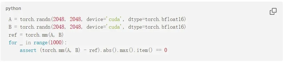
So why doesn’t this test exhibit non-determinism?
To truly understand the source of non-determinism in LLM inference, we must delve deeper.
Unfortunately, even defining what “deterministic LLM inference” means can be challenging. It might seem contradictory, but the following statements can all be true simultaneously:
- Some kernels on GPUs are non-deterministic.
- However, all kernels used during an LLM’s forward pass are deterministic.
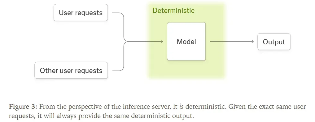
- Furthermore, the forward pass of an LLM inference server, like vLLM, can be considered deterministic.
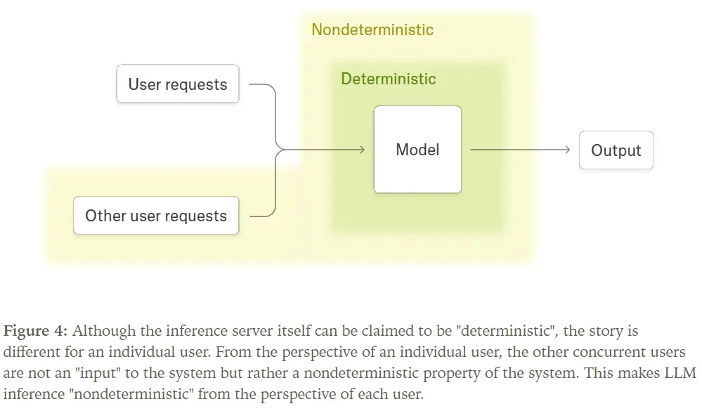
- Yet, from the perspective of any user interacting with the inference server, the results are non-deterministic.
In this article, we will explain why the “Concurrency + Floating-point” hypothesis falls short, reveal the true culprit behind LLM inference non-determinism, and demonstrate how to overcome it to achieve truly reproducible results.
The Original Sin: Floating-Point Non-Associativity
Before discussing non-determinism, it’s crucial to understand why numerical differences arise. We often conceptualize machine learning models as mathematical functions adhering to structural rules like commutativity and associativity. Shouldn’t our ML libraries provide mathematically sound results?
The culprit is floating-point non-associativity. That is, for floating-point numbers a, b, and c:
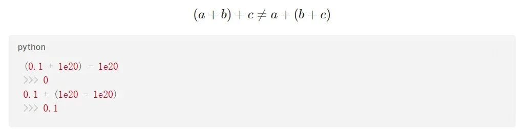
Ironically, it’s this break from associativity that makes floating-point numbers so useful.
Floating-point numbers allow for dynamic precision. For illustration, let’s use decimal (instead of binary) representation, where a floating-point number is formatted as: Mantissa * 10^Exponent. We’ll use a 3-digit mantissa and a 1-digit exponent. (Note: In computer science, the mantissa, or significand, is the part of a floating-point number that represents precision, determining the number of significant digits and accuracy.)
For example, the value 3450 can be precisely represented as $3.45 \times 10^3$. Smaller values like $0.486$ can be represented as $4.86 \times 10^-1$. This allows floating-point numbers to represent both extremely small and very large values, maintaining a constant number of significant digits.
If two floating-point numbers share the same exponent, their addition behaves much like integer addition:
![]()
But what happens if two floating-point numbers have different exponents, like 1230 and 23.4? Theoretically, their sum is 1253.4. However, due to the 3-digit mantissa limit, the result is rounded to $1.25 \times 10^3$ (or 1250).
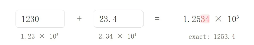
1230 requires 3 significant digits, and 23.4 also requires 3 significant digits. However, their sum (1253.4) needs 5 significant digits for exact representation. Consequently, our floating-point format must discard the last two digits (34). In essence, this is akin to rounding 23.4 to 20.0 before the addition.
This process leads to information loss. This occurs whenever we add floating-point numbers with different exponents. In practice, we frequently perform such additions. If we could guarantee that all floating-point numbers had the same exponent, we could simply use integers!
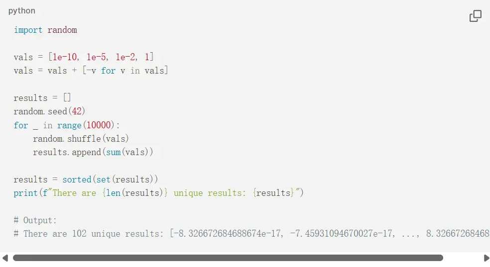
In other words, the order in which floating-point numbers are added can lead to entirely different results. In an extreme case, summing an array of numbers in different orders could yield 102 distinct outcomes.
While this is the fundamental reason for inconsistent outputs, it doesn’t directly explain the source of non-deterministic behavior. It also doesn’t help us understand why the order of floating-point addition changes, when this happens, or how we can avoid it.
The answer lies in the implementation of kernels.
Why Isn’t the Order of Addition in Kernel Computations Always Fixed?
As previously mentioned, a common explanation for inconsistent addition order in kernel computations is the “Concurrency + Floating-point” hypothesis.
This hypothesis suggests that if the execution order of concurrent threads is unpredictable, and accumulation operations depend on this order (e.g., atomic adds), the final accumulated result becomes unpredictable.
Confusingly, while this phenomenon can lead to non-deterministic kernel computations, concurrency mechanisms (and atomic adds) are not actually responsible for the non-determinism observed in large language model inference!
To explain the true culprit, we must first understand why modern GPU kernels rarely require atomic adds.
When Are Atomic Adds Necessary?
GPUs execute programs concurrently across multiple cores (streaming multiprocessors). Without built-in synchronization between these cores, communication can be problematic. For instance, if all cores need to accumulate into the same element, atomic adds (sometimes called fetch-and-add) are used. Atomic adds are inherently non-deterministic, as the order of accumulation depends entirely on which core finishes first.
Specifically, imagine summing a 100-element vector using 100 cores (e.g., torch.sum()). While elements can be loaded in parallel, the results must eventually be consolidated into a single value. One implementation approach uses atomic adds, where the hardware guarantees all additions occur but not in a specific order.

Atomic add operations ensure that each core’s computation contributes to the total sum. However, they do not guarantee the order of accumulation. This order depends on which core finishes first, leading to non-deterministic behavior.
Consequently, executing the same parallel program multiple times can yield different results. This is often what’s meant by run-to-run nondeterminism: executing the exact same Python script twice, even with identical library versions, may produce different outcomes.
While concurrent atomic add operations can make kernel execution unpredictable, they are not necessary for most kernels.
In fact, during a typical LLM forward pass, atomic adds are generally not required. This might be surprising, as reduction operations in parallel computation often benefit from atomic adds. However, atomic adds are typically unnecessary for two primary reasons:
- Parallelism along the batch dimension is often sufficient, eliminating the need for parallelization along the reduction dimension.
- Over time, most neural network libraries have adopted strategies to achieve predictable results without sacrificing performance.
Due to these factors, omitting atomic adds incurs minimal performance penalty for the vast majority of neural network operations.
Naturally, a few common operations do experience significant performance degradation without atomic adds. An example is scatter_add in PyTorch (a[b] += c). However, the only commonly used operation in LLMs that relies on atomic adds is the backward pass of FlashAttention.
Crucially, the forward pass of LLMs involves no operations requiring atomic adds. Therefore, the forward pass process itself is run-to-run deterministic (i.e., produces consistent results across runs).
Wikipedia defines a deterministic algorithm as one that, given a specific input, always produces the same output. Here, as long as the input is identical (i.e., the inference server processes the exact same request), the forward pass will consistently generate the same output.
However, a deterministic forward pass does not imply a deterministic overall system. For instance, if a request’s output depends on concurrently processed requests (like batch_norm), the LLM inference process becomes non-deterministic from the perspective of a single request. This is because each request cannot predict the content of other concurrent requests.
It turns out that our request outputs do depend on concurrently processed user requests. This isn’t due to cross-batch information leakage but rather a lack of batch invariance in our forward pass, causing the output for a given request to be influenced by variations in the batch size during the forward pass.
Batch Invariance and Determinism
To illustrate batch invariance, let’s simplify the problem and focus solely on matrix multiplication (matmul). We can assume all matmul implementations are run-to-run deterministic, meaning they produce the same result for the same input every time.
However, they are not batch invariant. In other words, as the batch size changes, individual elements within the batch may experience different computational outcomes.
Mathematically, this is quite anomalous. Theoretically, matrix multiplication should be independent across the batch dimension; the presence or size of other elements in the batch should not affect the computation of a specific element.
Yet, experimental evidence shows this is not the case.
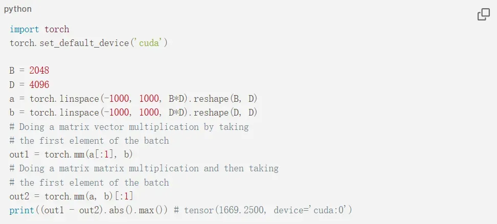
Note that “determinism” here refers to the consistency of results across multiple runs. If you execute this script repeatedly, it will consistently return the same output.
However, when a non-batch-invariant kernel is used as part of a larger inference system, the entire system can become non-deterministic. When you send a request to an inference endpoint, the server’s load is unpredictable from the user’s perspective. This load dictates the kernel’s batch size, which in turn influences the final outcome for each request.
Combining a kernel property that is not invariant to batch size with the inherent uncertainty of that property (e.g., server load) results in a non-deterministic system.
In essence, the primary reason why almost all large language model inference endpoints are non-deterministic is the uncertainty of the load (and consequently, the determined batch size)! This uncertainty is not exclusive to GPUs; LLM inference endpoints running on CPUs or TPUs face the same challenges. Therefore, to avoid non-determinism in inference servers, we must ensure that kernels are invariant to batch size.
To understand how to achieve this, we first need to examine why kernels are not batch-invariant by default.
How Can We Make Kernels Batch-Invariant?
To ensure Transformer model implementations are independent of batch size, we must guarantee that each core module within the model is batch-invariant. Fortunately, we can assume that all pointwise operations are batch-invariant. Thus, we only need to consider three operations: RMSNorm, matrix multiplication, and attention.
Coincidentally, the complexity of these operations increases sequentially. Achieving batch invariance for each requires specific considerations while maintaining reasonable performance. Let’s start with RMSNorm.
RMSNorm Implementation:
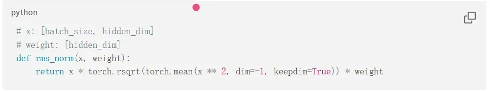
The requirement for batch invariance is that, regardless of a kernel’s batch size, the reduction order for each element must remain consistent. It’s important to note that this doesn’t mandate using the same reduction strategy every time. For example, even if we change the number of elements being reduced, as long as the reduction order remains consistent, our algorithm still adheres to batch invariance.
Therefore, batch invariance is only violated when the batch size influences the reduction strategy.
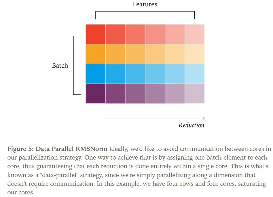
Let’s examine the standard parallelization strategy for RMSNorm. Generally, parallel algorithms benefit from minimizing communication between cores. For simplicity here, assume “cores” refer to SMs (Streaming Multiprocessors). More specifically, the critical property is that the number of thread blocks launched by the kernel exceeds the number of SMs.
Based on this, one viable strategy is to assign each batch element to a core, as depicted in the figure.
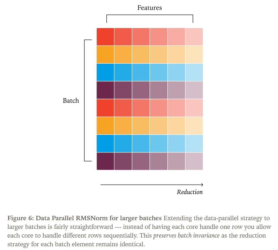
When we increase the batch size, it doesn’t affect the reduction strategy; if a batch size of 200 provides sufficient parallelism for the kernel, a batch size of 2000 clearly does too.
On the other hand, decreasing the batch size presents challenges. Since we allocate one core per batch element, a smaller batch size means more cores than batch elements, leading to idle cores. In such scenarios, skilled kernel engineers employ solutions like atomic adds or segmented reduction to maintain good parallelism and boost performance. However, this alters the summation strategy, rendering the kernel non-batch-invariant.
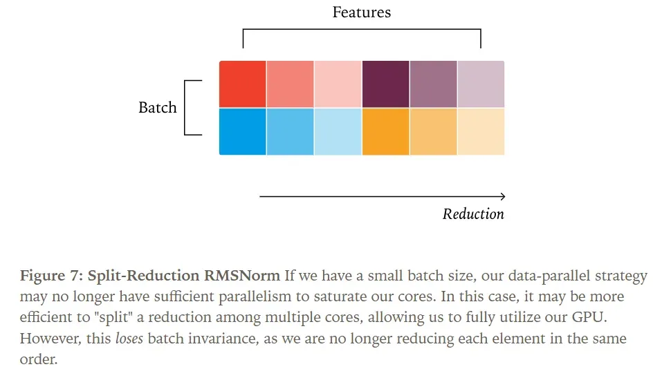
The simplest solution is to simply ignore these cases. This isn’t entirely unreasonable, as kernels usually execute quickly with very small batch sizes, so even a performance dip won’t be catastrophic.
If we must optimize for this scenario, one approach is to always use a reduction strategy that provides sufficient parallelism even at minimal batch sizes. Such a strategy might lead to over-parallelization at larger batch sizes, preventing peak performance, but it ensures acceptable (though not optimal) performance across the entire range of batch sizes.
Batch-Invariant Matrix Multiplication
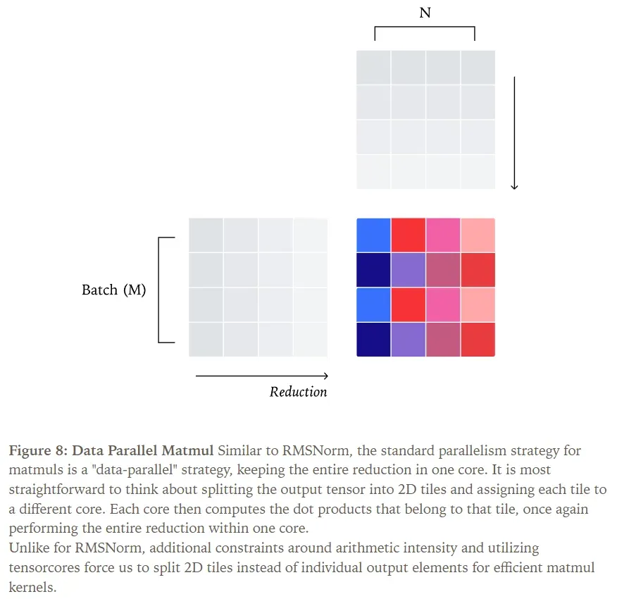
Essentially, matrix multiplication can be viewed as a series of pointwise operations followed by a reduction. If we parallelize matrix multiplication by partitioning the output into small tiles, we achieve a data-parallel kernel strategy where each reduction occurs within a single core.
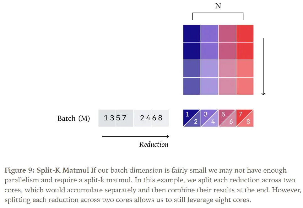
Similar to RMSNorm, the batch dimensions (M and N) of matrix multiplication can become too small, forcing us to split along the reduction dimension (K). Despite having two batch dimensions, matrix multiplication still requires substantial work per core to effectively utilize Tensor Cores. For example, a matrix multiplication of [1024, K] x [K, 1024] with a standard [128, 128] 2D tile size would, with a data-parallel strategy, only distribute across at most 64 cores—insufficient to saturate a GPU.
Splitting along the reduction dimension in matrix multiplication is known as Split-K matrix multiplication. As with RMSNorm, employing this strategy breaks batch invariance.
Matrix multiplication has an additional complexity: Tensor Core instructions. For reduction operations, we can process one row at a time; however, efficient matrix multiplication kernels must process an entire tile at once.
Each Tensor Core instruction (e.g., wgmma.mma_async.sync.aligned.m64n128k16) may have different internal reduction orders. One reason to choose a different Tensor Core instruction might be a very small batch size. For instance, if our Tensor Core PTX instruction operates on a tile of length 256, but the batch size is only 32, we’re wasting almost all computational resources! When the batch size is 1, the fastest kernels often don’t use Tensor Cores at all.
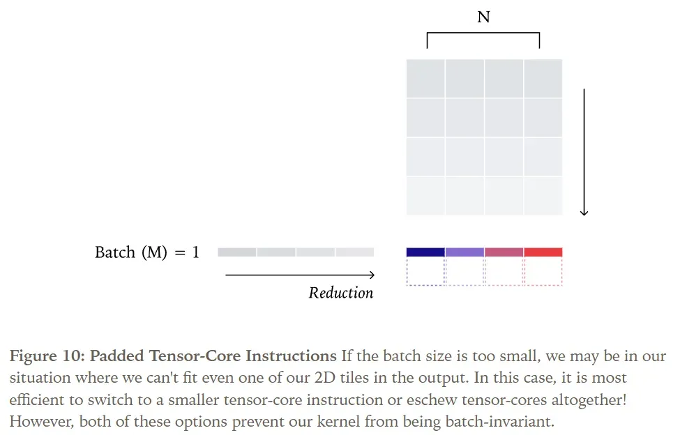
Therefore, the simplest way to ensure batch-invariant matrix multiplication is to compile a fixed kernel configuration and use it for all shape calculations. While this incurs some performance loss, it is usually not catastrophic in LLM inference scenarios. Notably, the Split-K strategy is most needed when M and N dimensions are small, and fortunately, in our application, the N dimension (model dimension) is typically quite large!
Batch-Invariant Attention Mechanism
After achieving batch invariance in matrix multiplication, the attention mechanism introduces two additional challenges—fittingly, as it involves two matrix multiplications.
- Unlike RMSNorm and matrix multiplication, which only reduce along the feature dimension, the attention mechanism now requires reduction along both feature and sequence dimensions.
- Consequently, the attention mechanism must accommodate various inference optimizations that affect sequence processing (e.g., paged attention, KV caching).
Therefore, to achieve determinism in LLM inference, our numerical computations must remain invariant to two factors: the number of requests processed concurrently, and how each request is partitioned within the inference engine.
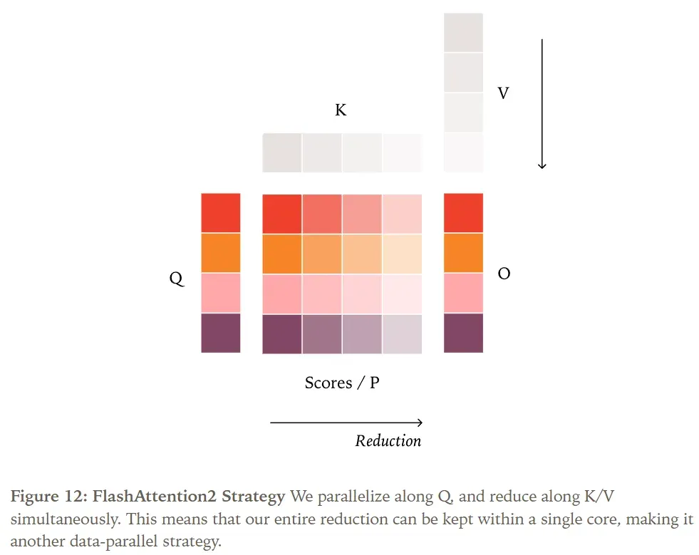
Let’s first examine the standard parallel strategy for attention, initially proposed by FlashAttention-2. Similar to RMSNorm and matrix multiplication, its default strategy is data parallelism. Since the reduction occurs along the Key/Value (K/V) tensors, data parallelism can only parallelize along the Query (Q) tensor.
For example, depending on the inference engine’s choice, a sequence might be processed in parts (as in paged attention) or all at once (if prefilling is contiguous). To achieve batch invariance, the reduction order for a given token must be independent of the number of other tokens in its sequence being processed concurrently.
This goal is unachievable if you reduce the K/V values in the KV cache separately from the K/V values of the token currently being processed (as done in vLLM’s Triton attention kernels). For instance, when processing the 1000th query token in a sequence, the reduction order must be identical whether there are 0 tokens in the KV cache (prefill phase) or 999 tokens (decoding phase).
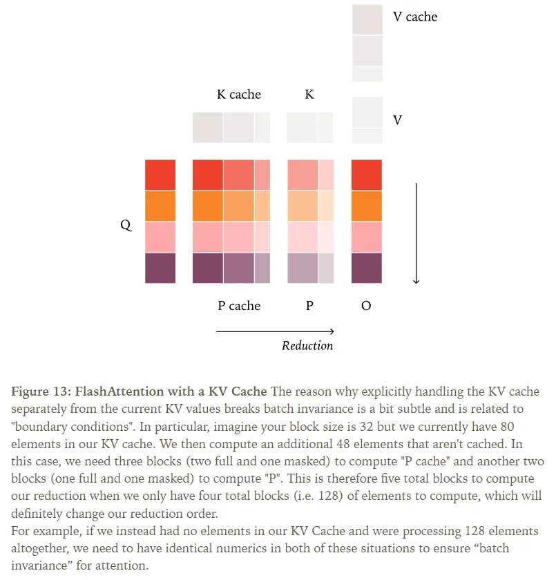
To address this, we can update the KV cache and page tables before the attention kernel runs, ensuring our keys and values maintain a consistent memory layout regardless of the number of tokens processed.
With this added processing (and all prior measures like using consistent tile sizes), we can achieve a batch-invariant attention mechanism!
However, there’s a critical issue here. Unlike matrix multiplication, attention computations in LLM inference often do require a split-reduction kernel—often referred to as Split-KV or FlashDecoding. This is because if we don’t parallelize along the reduction dimension, we can only parallelize along the batch, head, and query length dimensions.
During the decoding phase of attention, the query length is very small (typically 1), so unless the batch size is extremely large, we often cannot saturate the GPU. Unfortunately, this scenario is not as easily disregarded as in RMSNorm and matrix multiplication. For instance, if your KV cache is very long, the attention kernel computation can take a significant amount of time even for a single request.
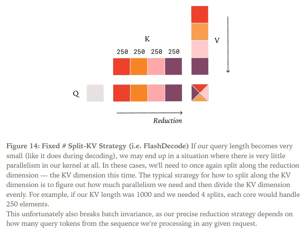
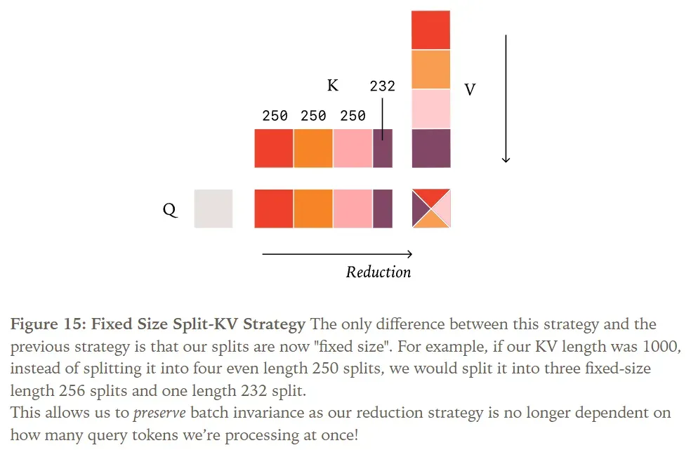
Furthermore, the split-reduction strategy commonly used for attention also poses challenges for batch invariance. For example, FlashInfer’s balanced scheduling algorithm selects the maximum split size to saturate all GPU cores, making its reduction strategy non-batch-invariant. However, unlike RMSNorm/matrix multiplication, simply choosing a fixed number of splits is insufficient regardless of batch size.
Instead, to achieve batch invariance, we must adopt a fixed split size strategy. In other words, we fix the size of each split chunk, not the number of splits, ultimately resulting in a variable number of splits. This way, we guarantee that regardless of how many tokens are being processed, we always perform the exact same reduction order.
Implementation
Leveraging vLLM and its FlexAttention backend, along with torch.Library, we provide a demonstration of deterministic inference. torch.Library allows us to replace most relevant PyTorch operators in a non-intrusive manner.
You can find the “batch-invariant” kernel library and a vLLM example running in “deterministic” mode at:
Link: https://github.com/thinking-machines-lab/batch_invariant_ops
Experiments
How Uncertain Are the Completed Results?
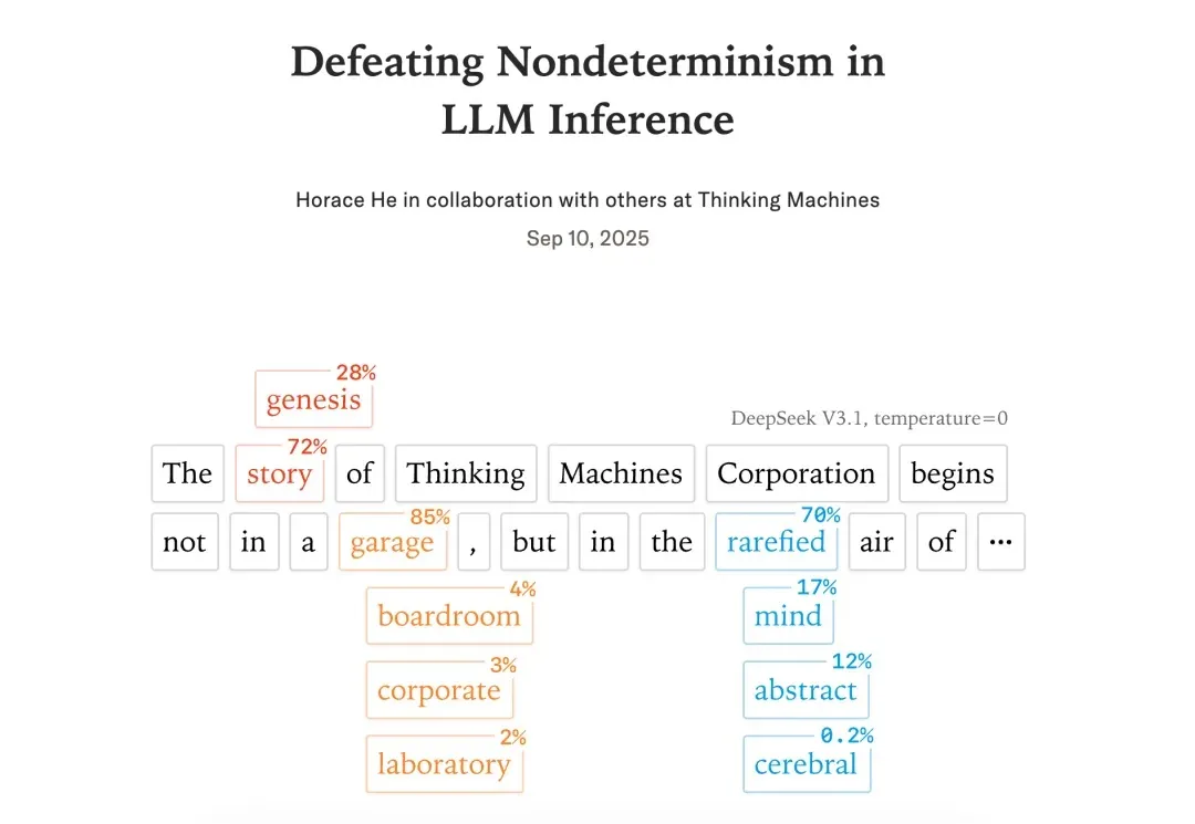
Using the Qwen3-235B-A22B-Instruct-2507 model, we sampled 1000 completions with temperature set to 0, using the prompt “Tell me about Richard Feynman” (in non-chain-of-thought mode), generating 1000 tokens per completion.
Astonishingly, we obtained 80 distinct completions, with the most frequent appearing 78 times.
Upon examining the differences, we found that the results were actually identical for the first 102 tokens!
The first divergence occurred at the 103rd token. All results generated the sequence “Feynman was born on May 11, 1918, in”. However, subsequently, 992 completions generated “Queens, New York,” while the remaining 8 produced “New York City.”
However, once we enabled the batch-invariant kernels, all 1000 completions became identical. This is precisely the behavior a sampler should exhibit, but achieving deterministic results is impossible without our batch-invariant kernels.
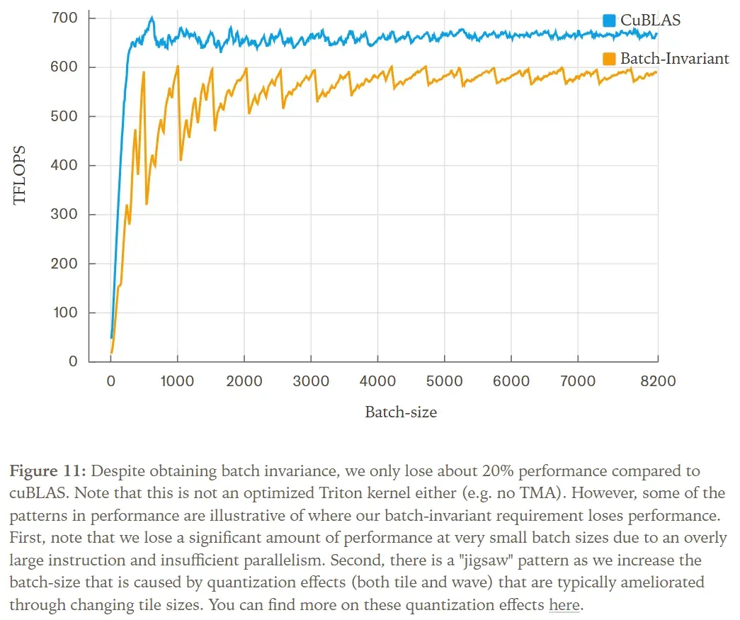
Performance
We have not yet focused on optimizing the performance of the batch-invariant kernels. However, we conducted some experiments to verify that their performance remains within an acceptable range.
We set up an API server with a single GPU, running the Qwen-3-8B model, and requested 1000 sequences with output lengths between 90 and 110 tokens.
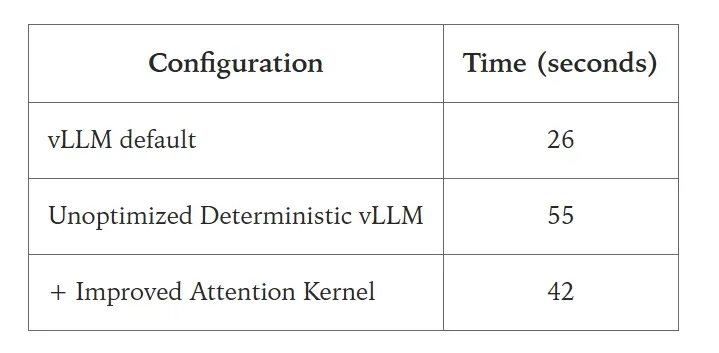
The primary performance degradation stems from the fact that the FlexAttention integration within vLLM is not yet deeply optimized. Nevertheless, we observed no catastrophic performance decline.
True On-Policy Reinforcement Learning
As researchers have pointed out, numerical discrepancies between training and inference implicitly transform our on-policy reinforcement learning (RL) into off-policy RL.
Of course, if we cannot even obtain identical results from two identical inference requests, achieving identical results between training and inference becomes impossible. Thus, deterministic inference enables us to modify the training stack to obtain identical results between sampling and training, ultimately enabling true on-policy RL.
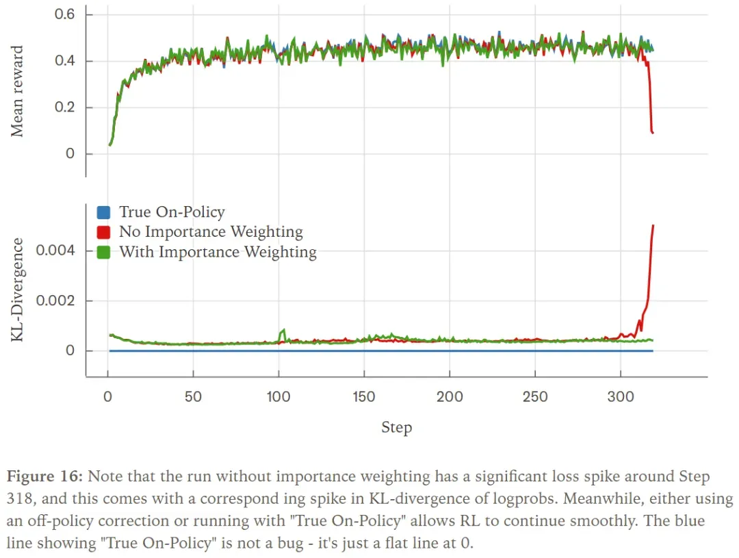
We experimented with the RLVR setup on Bigmath, where the RL policy was initialized with the Qwen 2.5-VL instruct 8B model, with a maximum rollout length of 4096.
Without training with off-policy correction (i.e., importance weighting), our rewards collapsed mid-training. Adding the off-policy correction term allowed training to proceed smoothly. However, if we achieve identical results between the sampler and the trainer, we are entirely in an on-policy state (i.e., KL divergence is 0) and can also train smoothly.
We can also plot the KL divergence of log probabilities between the sampler and trainer, where all 3 runs exhibited significantly different behavior. When running with importance weighting, the KL divergence remained around 0.001 with occasional spikes. However, running without importance weighting resulted in KL divergence peaking around the same time as the reward collapse. Naturally, when running “true on-policy RL,” our KL divergence remained consistently at 0, indicating no discrepancy between the training and sampling policies.
Conclusion
Modern software systems are often composed of many layers of abstraction. In machine learning, when we encounter non-determinism and subtle numerical differences, there’s a tendency to simply overlook them.
After all, our systems are inherently “probabilistic”—what’s a little more uncertainty? When unit tests fail, what’s wrong with increasing atol/rtol? Surely, differences in log probabilities between the trainer and sampler aren’t real bugs, are they?
We reject this passive mindset. With just a bit more effort, we can understand the roots of non-determinism and, more importantly, solve them!
We hope this blog post provides the community with a robust framework for tackling non-determinism in inference systems and inspires more individuals to delve deeply into understanding their own systems.